what happens to the shape of the chi-square distribution as the df value increases?

Learning Objectives

1. Understand the characteristics of the chi-square distribution
2. Carry out the chi-foursquare examination and translate its results
3. Empathise the limitations of the chi-square test

Key Terms

Chi-Square Distribution: a family asymmetrical, positively skewed distributions, the exact shape of which is determined by their respective degrees of freedom
Observed Frequencies: the cell frequencies actually observed in a bivariate table
Expected Frequencies: The cell frequencies that one might expect to see in a bivariate table if the two variables were statistically contained

Overview

The primary employ of the chi-foursquare test is to examine whether two variables are independent or not. What does it mean to be independent, in this sense? It ways that the two factors are not related. Typically in social science research, we're interested in finding factors that are dependent upon each other—instruction and income, occupation and prestige, age and voting behavior. Past ruling out independence of the two variables, the chi-square can be used to assess whether two variables are, in fact, dependent or not. More than generally, we say that i variable is "not correlated with" or "independent of" the other if an increase in one variable is not associated with an increase in the another. If two variables are correlated, their values tend to move together, either in the same or in the contrary direction. Chi-square examines a special kind of correlation: that between two nominal variables.

The Chi-Square Distribution

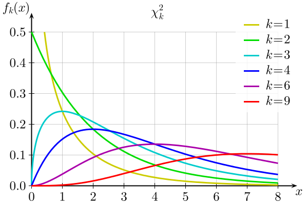
The chi-square distribution, like the t distribution, is actually a serial of distributions, the exact shape of which varies according to their degrees of freedom. Different the t distribution, however, the chi-foursquare distribution is asymmetrical, positively skewed and never approaches normality. The graph beneath illustrates how the shape of the chi-square distribution changes as the degrees of freedom (k) increase:

The Chi-Foursquare Examination

Earlier in the semester, you familiarized yourself with the five steps of hypothesis testing: (1) making assumptions (2) stating the aught and inquiry hypotheses and choosing an alpha level (three) selecting a sampling distribution and determining the test statistic that corresponds with the called alpha level (4) calculating the exam statistic and (five) interpreting the results. Like the t tests we discussed previously, the chi-square test begins with a scattering of assumptions, a pair of hypotheses, a sampling distribution and an alpha level and ends with a conclusion obtained via comparison of an obtained statistic with a critical statistic. The assumptions associated with the chi-foursquare test are fairly straightforward: the data at paw must have been randomly selected (to minimize potential biases) and the variables in question must exist nominal or ordinal (there are other methods to exam the statistical independence of interval/ratio variables; these methods will exist discussed in subsequent chapters). Regarding the hypotheses to be tested, all chi-square tests have the same full general null and inquiry hypotheses. The zero hypothesis states that there is no relationship between the ii variables, while the enquiry hypothesis states that there is a human relationship betwixt the two variables. The examination statistic follows a chi-square distribution, and the conclusion depends on whether or not our obtained statistic is greater that the critical statistic at our chosen alpha level.

In the following case, we'll use a chi-square test to determine whether in that location is a relationship betwixt gender and getting in trouble at schoolhouse (both nominal variables). Beneath is the table documenting the raw scores of boys and girls and their respective behavior problems (or lack thereof):

Gender and Getting in Trouble at Schoolhouse

	Got in Problem	Did Non Get in Trouble	Total
Boys	46	71	117
Girls	37	83	120
Total	83	154	237

To examine statistically whether boys got in trouble in school more often, nosotros need to frame the question in terms of hypotheses. The null hypothesis is that the two variables are independent (i.east. no relationship or correlation) and the research hypothesis is that the two variables are related. In this instance, the specific hypotheses are:

H0: There is no relationship between gender and getting in trouble at schoolhouse
H1: There is a human relationship between gender and getting in trouble at school

As is customary in the social sciences, we'll ready our alpha level at 0.05

Next we need to calculate the expected frequency for each cell. These values stand for what we would expect to run across if there really were no human relationship betwixt the two variables. Nosotros calculate the expected frequency for each cell by multiplying the row total by the cavalcade total and dividing by the total number of observations. To get the expected count for the upper right cell, we would multiply the row total (117) by the column full (83) and carve up by the total number of observations (237). (83 x 117)/237 = 40.97. If the 2 variables were independent, we would expect 40.97 boys to get in trouble. Or, to put it some other way, if there were no relationship betwixt the two variables, we would wait to come across the number of students who got in trouble be evenly distributed beyond both genders.

We practise the same thing for the other three cells and finish up with the following expected counts (in parentheses next to each raw score):

Gender and Getting in Problem at School

	Got in Trouble	Did Not Make it Problem	Full
Boys	46 (40.97)	71 (76.02)	117
Girls	37 (42.03)	83 (77.97)	120
Total	83	154	237

With these sets of figures, nosotros calculate the chi-square statistic as follows:

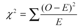
For each cell, nosotros square the divergence between the observed frequency and the expected frequency (observed frequency – expected frequency) and split up that number by the expected frequency. And then nosotros add together all of the terms (in that location volition be four, i for each cell) together, like so:

Subsequently nosotros've crunched all those numbers, we cease up with an obtained statistic of 1.87. (Please note: a chi-foursquare statistic can't exist negative because nominal variables don't have directionality. If your obtained statistic turns out to be negative, you might want to check your math.) Only before we can come to a conclusion, we need to discover our disquisitional statistic, which entails finding our degrees of liberty. In this example, the number of degrees of freedom is equal to the number of columns in the table minus one multiplied by the number of rows in the table minus one, or (r-one)(c-1). In our example, nosotros take (2-one)(2-1), or 1 degree of freedom.

Finally, we compare our obtained statistic to our critical statistic constitute on the chi-foursquare table posted in the "Files" department on Canvas. We also need to reference our blastoff, which we set up at .05. As you can run into, the disquisitional statistic for an blastoff level of 0.05 and one degree of freedom is 3.841, which is larger than our obtained statistic of 1.87. Because the critical statistic is greater than our obtained statistic, we can't reject our null hypothesis.

The Limitations of the Chi-Foursquare Examination

There are 2 limitations to the chi-square test well-nigh which you should exist enlightened. First, the chi-square test is very sensitive to sample size. With a big enough sample, fifty-fifty trivial relationships tin appear to exist statistically meaning. When using the chi-square test, you should go along in mind that "statistically significant" doesn't necessarily hateful "meaningful." Second, remember that the chi-foursquare can only tell united states of america whether two variables are related to one another. Information technology does not necessarily imply that one variable has any causal effect on the other. In order to establish causality, a more detailed assay would be required.

Chief Points

• The chi-foursquare distribution is actually a serial of distributions that vary in shape according to their degrees of freedom.
• The chi-square test is a hypothesis examination designed to examination for a statistically significant human relationship between nominal and ordinal variables organized in a bivariate table. In other words, it tells us whether 2 variables are contained of i another.
• The obtained chi-square statistic essentially summarizes the difference betwixt the frequencies really observed in a bivariate tabular array and the frequencies we would expect to see if in that location were no relationship between the two variables.
• The chi-square examination is sensitive to sample size.
• The chi-square exam cannot plant a causal relationship between two variables.

Carrying out the Chi-Square Exam in SPSS

To perform a chi foursquare test with SPSS, click "Clarify," and so "Descriptive Statistics," and so "Crosstabs." As was the instance in the terminal chapter, the independent variable should exist placed in the "Columns" box, and the dependent variable should be placed in the "Rows" box. Now click on "Statistics" and check the box next to "Chi-Square." This test volition provide evidence either in favor of or against the statistical independence of two variables, but it won't give you lot whatsoever information near the forcefulness or direction of the relationship.

After looking at the output, some of you are probably wondering why SPSS provides yous with a 2-tailed p-value when chi-square is ever a one-tailed test. In all honesty, I don't know the answer to that question. However, all is not lost. Considering two-tailed tests are always more bourgeois than i-tailed tests (i.e., it's harder to pass up your null hypothesis with a two-tailed examination than it is with a one-tailed test), a statistically pregnant upshot under a two-tailed supposition would besides exist significant nether a ane-tailed assumption. If you're highly motivated, y'all can compare the obtained statistic from your output to the critical statistic found on a chi-square chart. Here's a video walkthrough with a slightly more detailed explanation:

Exercises

1. Using the World Values Survey data, run a chi-square exam to decide whether there is a human relationship betwixt sex ("SEX") and marital status ("MARITAL"). Written report the obtained statistic and the p-value from your output. What is your conclusion?
2. Using the Add Wellness data, run a chi-square exam to decide whether at that place is a relationship between the respondent's gender ("GENDER") and his or her grade in math ("MATH"). Again, report the obtained statistic and the p-value from your output. What is your determination?

bergmanfaspen.blogspot.com

Source: https://soc.utah.edu/sociology3112/chi-square.php

Share this post